Regression methods model the relationship between independent and dependent variables. Linear regression models are widely used; however, they may not be suitable when the relationship between variables isn’t linear. Polynomial regression is an alternative that models the relationship of the dependent variable as a polynomial function of the independent variable.

This post (from Armancomputer blog) will provide an overview of polynomial regression and its applications in modeling paired or multidimensional data. Additionally, we will demonstrate the performance of this regression technique by implementing it in the R programming language and using a practical example with real-world data.

Polynomial regression

At times, a “Non-Linear” model involving descriptive and response variables can be represented as a polynomial of the kth degree. “Polynomial Regression” models are particularly adept at capturing the relationship between predictor and dependent variables in such instances.

It is known that the equation of a straight line can be determined by two distinct points on that line. Indeed, in Euclidean space, only one straight line can intersect two points. Similarly, to define a 2nd degree curve, knowing three points on the curve is sufficient to derive the corresponding equation, including the parameters that define the equation and its shape.

The greater the number of points, the higher the degree of the curve or polynomial that can pass through those points. It appears that the degree of the curve or polynomial is consistently one less than the number of points. Consequently, to fit a curve to 10 points, a 9th degree polynomial is required, which inherently has a high complexity due to its 10 parameters. A polynomial function or relation of order k is typically expressed in the following manner.

$$\large f(x) = a_0 + a_1 x+ a_2 x^2 + a_3 x^3 + \ldots + a_k x^k$$

Polynomial regression aims to estimate the parameters of a polynomial or regression using far fewer variables than data points. This reduces the model’s complexity but introduces errors. Thus, it strikes a balance between overfitting and underfitting within the model.

Taylor’s theorem, or expansion, allows us to express any “continuous function” with multiple derivatives in terms of a linear or polynomial relationship, which is the basis for polynomial regression.

In the depicted scenario, the green line represents the linear regression model, while the red line illustrates the second-order polynomial model. Evidently, the red curve more accurately captures the variations of the response variable.

 

 

In this way, the following linear regression model can be considered for polynomial regression.

$$\large y = \beta_0 + \beta_1 X + \beta_2 X^2 + \ldots + \beta_k X^k + \epsilon$$

Based on this, polynomial regression can be inserted as multiple linear regression in the following form.

$$\large X_1 = X , \; \; X_2 = X^2, \; \; \ldots , \; \; X_k = X^k$$

Running polynomial regression in R

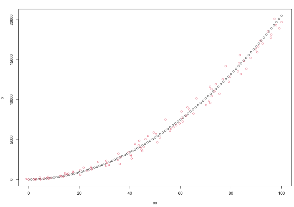
To run polynomial regression, we simulate a dataset which contains the values that have quadratic relation.

The following codes have been created in order to perform polynomial regression based on the dependent variable (y) and the independent variable (x,$x^2$). So we add some noise to simulated data to show the non-deterministic relation between dependent and independent variables.

Note: It is obvious that there is a high correlation between x and $x^2$ and maybe collinearity and variance inflation will be accrued in our model.

Here is the output of running code

In order to compare the simple linear regression model and the polynomial model, we use the lm function twice, which performs the fitting of the linear regression model. In the first case, we will store the result of the model in the simple_linear_model variable and when we use the 2nd order polynomial regression (using poly function), we will store the output in the rawpolynomial_model variable.

The result of executing the codes and building the linear model (first model) will be as follows.

As you can see, in simple_linear_mode, the value of the origin (Intercept) is equal to -819.686 and coefficient for independent variable (x) is 104.772. They are too far from true values (3=constant, and 5= coefficient). But it is interesting that they are all significant.

In other model (using polynomial with degree 2) the R code is as follows:

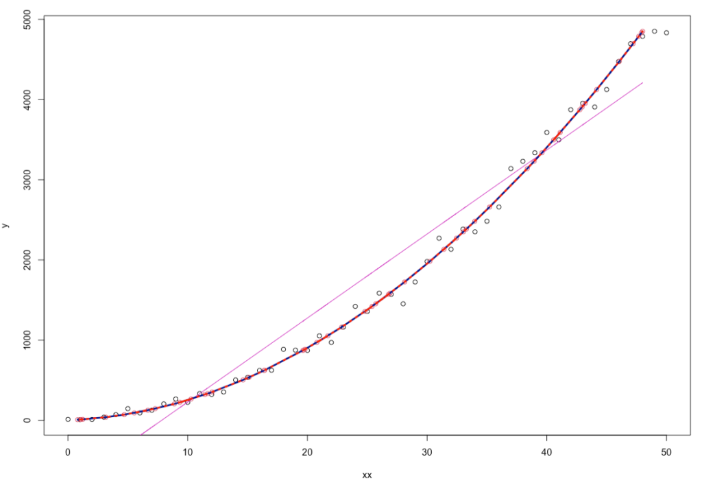
We used poly function to make the quadratic form. the parameter RAW shows that we use the squared values of x ($x^2$) to produce quadratic form. The output shows the models characteristics and plot shows the good fit to quadratic curve.

Here, the intercept is changed to -16.76 and coefficients for x and $x^2$ are 9.22 and 1.92 respectively (round to 2 decimal places). But again, all are significant unless intercept.

The correlation between x and $x^2$ is equal to 0.96 that shows the collinearity problem.

Note: Function poly produces orthogonal polynomial if raw parameter is equal to false (default).

To address the issue of collinearity, we employ the poly function to generate an orthogonal polynomial of degree 2, and then use these values to conduct a polynomial regression once more.

Note: For this example, the polynomial regression model can be done with degree or order three, but the number of parameters and thus the complexity of the model increases. The code related to this situation for polynomials of degree 3 and the resulting result can be seen below.

As you see, there is no collinearity, but coefficients are changed again.

Correlation between to independent variables is almost zero but plot of fitted curve (dotted red) is very near to previous one. All coefficients are significant.

Of course, in this section, you can see that the fitted values for all three models are also compared with each other. The difference between the predicted value in the first model and other models is very large, while between the second and third order models, the changes in prediction or error are not very significant.

Advantages and disadvantages of using polynomial regression

Estimation of polynomial regression parameters (such as polynomial degree) are usually done by trial and error or optimization methods, and appropriate solutions are obtained during the repetition of a process. Numerical calculation methods such as Gradient Descent, elbow method, Cross-validation and Interpolation Techniques are used in such cases.

Anyway, the advantages and disadvantages of polynomial regression can be listed as follows.

Advantages for polynomial regression

• Polynomial regression finds the best approximate model between dependent and independent variable.
• Many complex non-linear functions can be fitted by polynomial regression.
• Convergence to the optimal answer is often accompanied by high speed.

Disadvantages polynomial regression

• The presence of outlier data will cause the model to be misleading and as a result the fitted value will be invalid.
• Unfortunately, identifying outlier data in nonlinear models is more complex and difficult than linear models, which limits the use of polynomial regression.